How to conduct a simple name search

After installing the clusterpluck package, this tutorial demonstrates how to search for an open cluster using just its name.

First, import the module and classes.

import clusterpluck as cp
from clusterpluck.gaia import Refine, Info, Plotting
import warnings
warnings.filterwarnings("ignore")
%matplotlib inline

Then, perform the search, downloading the basic cluster data from the SIMBAD Astronomical Database and the individual star data from the Gaia archive. The default search is processed using Gaia DR2.

The name of the cluster must be in a string and must also be in a recognised format, i.e. M.. for Messier catalogue, NGC.. for New General Catalogue, etc. It is possible that lesser known catalogues can be used but they may cause an error if the format doesn’t match SIMBAD’s.

The results will be downloaded and stored as a CSV file.

cp.search_name('M47')

Number of stars: 992
RA: 07 36 35 Dec: -14 29.3 Rad: 0.5
PM_RA: -7.02 PM_Dec: 0.9592 PM_Rad: 2
Distance range: 242 pc to 725 pc

Messier 47 is an open cluster in Cancer. The output of the search contains the following information:

• The number of stars downloaded from the Gaia database.

• The right ascention (RA), declination (Dec) and search radius of the cluster. This is its position in the sky and it’s size.

• The proper motion RA, Dec and proper motion search radius. This is the rate of cluster’s apparent movement across the sky. Cluster stars will all share approximately the same apparent movement and so will form a tight group when these data are plotted.

• Finally, the distance range of the search. This helps filter out lots of stars that are unrelated but can also cause cluster stars to be lost. In particular any objects further than 1 kpc (1000 pc) away can suffer from this.

Any or all of these can be amended by using the general search() method but that is for another tutorial.

Now let’s use the load() method to load the data into a Pandas dataframe.

t = cp.load()

We can check the contents of the dataframe using simple pandas commands.

t.info()

<class 'pandas.core.frame.DataFrame'>
RangeIndex: 992 entries, 0 to 991
Data columns (total 20 columns):
 #   Column           Non-Null Count  Dtype
---  ------           --------------  -----
 0   name             992 non-null    object
 1   otypes           992 non-null    object
 2   parallax         992 non-null    float64
 3   parallax_error   992 non-null    float64
 4   pmra             992 non-null    float64
 5   pmra_error       992 non-null    float64
 6   pmdec            992 non-null    float64
 7   pmdec_error      992 non-null    float64
 8   bp_rp            992 non-null    float64
 9   phot_g_mean_mag  992 non-null    float64
 10  ra               992 non-null    float64
 11  dec              992 non-null    float64
 12  distance         992 non-null    float64
 13  distance_error   992 non-null    float64
 14  m_v_tycho        992 non-null    float64
 15  b_v              992 non-null    float64
 16  abs              992 non-null    float64
 17  t_k              992 non-null    float64
 18  lum_s            992 non-null    float64
 19  prob             992 non-null    float64
dtypes: float64(18), object(2)
memory usage: 155.1+ KB

As you can see the load() method takes some time to complete. That’s because it’s doing a lot of work. The parallax is converted into a distance in parsecs, the gaia g magnitude and colour index is converted into a more standardized Tycho magnitude and b - v colour index. From these the approximate stellar absolute magnitude, effective temperature and luminosity is calculated.

Then a simple cluster probability algorithm is run to help classify stars by giving them a percentage style ‘rating’ based on their proximity to the centeroids of the position, distance and proper motion of the cluster.

Finally, a matching algorithm runs through all the objects and compares their RA and DEC to a list of objects in the SIMBAD catalogue. If these match the name of the object and its object type is added to the dataframe and saved in CSV format.

The dataframe is in descending g (green) magnitude order.

t

	name	otypes	parallax	parallax_error	pmra	pmra_error	pmdec	pmdec_error	bp_rp	phot_g_mean_mag	ra	dec	distance	distance_error	m_v_tycho	b_v	abs	t_k	lum_s	prob
0	HD 60855	**|*|Em*|Be*|V*|IR|UV|X	2.077637	0.207615	-7.109151	0.155182	0.780030	0.133099	-0.118344	5.627999	114.016190	-14.492770	481.315959	43.727498	5.641895	-0.150834	-2.770256	11890.825947	1182.078739	79.900015
1	HD 61224	**|*|Em*|Be*|IR|UV	2.012069	0.106906	-7.138949	0.080708	1.145077	0.083712	0.081778	6.473912	114.411640	-14.440757	497.000887	25.074589	6.499310	-0.011235	-1.982476	9207.670048	572.182144	38.532447
2	HD 61017	X|**|*|IR	2.021288	0.100697	-7.310861	0.086194	0.785335	0.074871	-0.002212	6.655011	114.171852	-14.443610	494.734135	23.477293	6.673285	-0.069918	-1.798574	10152.913748	483.029546	80.101179
3	HD 61114	*|IR	1.743823	0.067370	-7.792587	0.054587	2.608254	0.045973	2.395475	6.861200	114.285469	-14.324596	573.452773	21.330566	8.088121	1.639623	-0.704367	2807.316771	176.315618	0.522240
4	HD 60998	*|UV|**|IR	1.865338	0.091669	-7.078137	0.070441	1.084258	0.063201	-0.031709	6.872384	114.150463	-14.484610	536.095954	25.111499	6.888938	-0.090495	-1.757274	10538.810106	465.000918	69.543404
...	...	...	...	...	...	...	...	...	...	...	...	...	...	...	...	...	...	...	...	...
987			2.101019	2.697285	-5.451604	1.943831	-0.055180	2.318828	1.512276	20.853565	114.108059	-14.141460	475.959477	267.552516	21.434158	1.004453	13.046308	3775.135396	0.000557	0.759856
988			3.006464	3.076210	-5.971694	2.067749	-0.149494	2.225318	1.086000	20.883945	114.298768	-14.845272	332.616656	168.215278	21.223415	0.699234	13.613695	4545.307747	0.000330	0.329157
989			3.919975	4.900724	-5.411766	3.079569	-0.184064	4.386642	1.416664	20.885458	114.524786	-14.436349	255.103698	141.733991	21.407289	0.935868	14.373705	3923.316770	0.000164	0.007395
990			4.023713	3.740082	-6.316390	3.189567	1.229143	2.255890	1.818579	20.899426	113.957239	-14.413898	248.526653	119.723675	21.684544	1.224519	14.707679	3369.758463	0.000121	0.539806
991			1.840975	3.254297	-5.187855	2.186801	2.466972	2.374998	3.004002	20.947468	114.296388	-14.796842	543.190356	346.929973	22.697336	2.076619	14.022576	2390.005509	0.000227	0.045637

992 rows × 20 columns

Once the data are loaded to a variable we can check to see if we have a cluster. Using the Refine class, let’s see how the proper motion plot, pm_plot(), looks.

Refine.pm_plot(t)

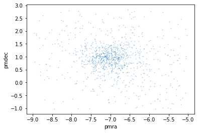
We can see the cluster’s stars are forming a group right in the middle of the plot. That means SIMBAD has given us good proper motion data and the default proper motion radius is acceptable. Any closer and we would lose relevent star data. Further away and there would be mnore chance of unrelated stars being included.

Now let’s look at a plot of the cluster as a star map, map().

Refine.map(t)

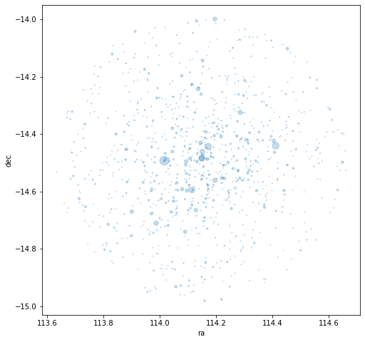
This plot shows a star map of the search with the star size proportional to their magnitude. It can help show us if our search radius is too wide or narrow. This looks pretty good as the cluster appears fully contained.

Now let’s see if the distance filter has correct values using the d_hist(). This produces a simple histogram of the stellar distances.

Refine.d_hist(t)

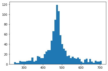
There is a very clear, tall peak in the middle of our graph that tells us the cluster stars are clearly outnumbering the unrelated stars. We can also see roughly how far away the cluster is in parsecs just by looking. The distance filter doesn’t need refining either. So that is all the parameters involved with the search.

However let’s have a look at two of the features we can draw from this data; a colour magnitude diagram and a more precise measurement of the distance.

Using the Plotting class, we can call the cmd() instance which uses values of g magnitude and the gaia bp-rp colour index…

Plotting.cmd(t)

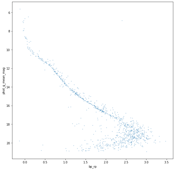
… and we have a beautiful CMD plot with the classic main sequence of stars running from top left to bottom right. These stars are in the middle of their lives, burning Helium in their cores in a relatively stable way just like our sun. The stars above the main sequence are mainly multiple star systems that have a slightly higher luminosity.

Other features are the brightest stars at the top which appear to just be ‘curling’ upwards. This is called the main sequence turn off. The stars here are running low on core Helium and starting to evolve into red giants. They’re not quite at that point but the position of the turn off is a major method of ageing clusters. At the other end are the red and white dwarfs.

Finally, use the Info class dist() instance to extract a calculated distance from the parallax data including a 2-sigma range.

Info.dist(t)

Distance: 474 pc
5%: 341 pc - 95%: 632